

Table of Contents
Background
Classification tasks can be useful for a wide range of activities including document classification and even medical diagnosis prediction. R happens to be a great tool by which one can essentially teach a computer to automatically classify documents by means of analyzing their content.
A Naive Bayes Classifier is a classic and simple machine learning technique based on Bayes’ Theorem, which in statistical inference is used to determine the probability that a given element belongs to a given class.
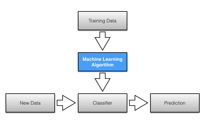
The term Supervised Learning refers to the fact that the algorithm classifies elements based on prior knowledge of the label to which related content was initially assigned, while the term Naive corresponds to the assumption that all the features in a dataset are independent from one another.
We won’t discuss the mathematical building blocks of Bayes’ law in this post, but we’ll focus instead on applying the theorem for document classification purposes, using the open source statistical programming language R.
Identifying the programming language of a file.
There are several reasons as to why someone would want to identify the programming language of a file, such as gathering static code metrics to assess the quality of a software unit.
One way to collect static metrics is to use parsers, which vary on the language a given file is written in. Knowing the programming language of a file thus helps ensure that the correct parser is used.
In this post, we will develop a Naive Bayes Classifier, which will take the text of a file as input, and provide a class label (type of language) as output.
Importing Data
1 - Loading Packages
We begin by loading the packages required for importing the data, namely readr, and will use dplyr, magrittr andpurrr to get it ready for our initial exploratory analysis.
library(dplyr)
library(magrittr)
library(purrr)
library(readr)
2 - Labelling Data
The files were sourced from Github, and saved in 4 separate directories.
Each directory contains files written in the vast majority in either Java, C, Python or JavaScript.
# Sourcing the Data

dir <- data.frame(directory = c("/Users/jckameni/Desktop/Data Science with R/guava/",
                                "/Users/jckameni/Documents/GitHub/node/test/",
                                "/Users/jckameni/Documents/GitHub/cpython",
                                "/Users/jckameni/Documents/GitHub/linux/drivers/"))
In Supervised Learning, we gather example input/output pairs (text/type) to help train the model.
# Function to label the data based on file extension.

list_files <- function(directory) {

df <- data.frame(doc_id =
                   list.files(directory, recursive = T, full.names = T, pattern =
                   ifelse(directory == "/Users/jckameni/Documents/GitHub/cpython", "\\.*py$",
                   ifelse(directory == "/Users/jckameni/Documents/GitHub/linux/drivers/", "\\.*c$",
                   ifelse(directory == "/Users/jckameni/Desktop/Data Science with R/guava/", "\\.*java$",
                   ifelse(directory == "/Users/jckameni/Documents/GitHub/node/test/", "\\.*js$", "")))),
                   ignore.case = F))
}
Preparing for Analysis
1 - Generating File List
In order to carry out an exploratory analysis, the data must be stored in a data frame.
The function above generates a table containing the files we will use for model training and testing purposes.
file_list <- apply(dir, 1, list_files) %>%
  purrr::map_dfr(
    magrittr::extract,
    'doc_id') %>%
  tbl_df() %>%
  distinct()
Now it would be interesting to have a look at what is inside of these files.
We can apply the read_delim() function from the readr package to extract the contents of the files as text and add them to our data frame.
first_df <- apply(file_list, 1, function(x) data.frame(text = paste(unlist(try(read_delim(x, delim = "\t"), silent = T)), collapse = " "),
                                         doc_id = x[1]))
2 - Final Data Frame
Here, we add a new column to the data frame and isolate the type (language) of the text using file extensions.
In this step, I gathered data which is known to contain one of the four programming languages that we are interested in.
final_df <- map_dfr(first_df, extract, c('doc_id', "text")) %>%
  mutate( type = ifelse(
    grepl(".java", doc_id, fixed = T),
    "Java", ifelse(
      grepl(".js", doc_id, fixed = T),
      "JavaScript", ifelse(
          grepl(".py", doc_id, fixed = T),
          "Python", ifelse(
              grepl(".c", doc_id, fixed = T),
              "C", "Other"
            ))
        )
      ))
  )) %>%
  group_by(type) %>%
  sample_n(1500, replace = T) %>%     # Sample 1500 files for each language
  distinct() %>%
  data.frame()
As we are now in possession of a dataset that we can work with, we can proceed with the exploratory analysis of the data.
The frame consists of 3 variables (doc_id, text , and type - the last of which corresponds to the language the file is written in).
3 - A Subset of the final data frame
## # A tibble: 3 x 1
##   `final_df[1:3, ]`$doc_id              $text                         $type
##   <chr>                                 <chr>                         <chr>
## 1 /Users/jckameni/Documents/GitHub/lin… /*  * RTC driver for the Mic… C
## 2 /Users/jckameni/Documents/GitHub/lin… " * Copyright (c) 2011 Broad… C
## 3 /Users/jckameni/Documents/GitHub/lin… " * Copyright 2012 Freescale… C
File count per language. (Table + Graph)
We load the ggplot2, ggthemes and plotly R libraries to perform some visualization.
library(ggplot2)
library(plotly)
library(ggthemes)
library(kableExtra)
library(knitr)
1 - Table
knitr::kable(type_count <- final_df %>%
  group_by(type) %>%
  summarise(count = n()), format = 'html' , caption = 'File Count per Programming Language') %>%
kable_styling(full_width = T)| type | count |
|---|---|
| C | 1431 |
| Java | 1181 |
| JavaScript | 1183 |
| Other | 70 |
| Python | 1028 |
2 - Graph
(language_count <- ggplotly(ggplot(final_df, aes(type)) +
                   geom_histogram(aes(fill = type), stat = 'count') + theme_economist_white() +
                   ggtitle("File count per Programming Language"), tooltip = c("x", 'count')))
Prediction Using Naive Bayes Classifier
- Loading
quantedapackage.
library(quanteda)A - Quantitative Text Analysis
- Shuffle the data
set.seed(2347)

final_df <- final_df[sample(nrow(final_df)),]- Construct Corpus from the text data.
lang_corpus <- corpus(final_df$text)- Attach variable
typeto the Corpus.
docvars(lang_corpus) <- final_df$type- Separate train and test data (70/30 split)
lang_train <- final_df[1:3385,]
lang_test <- final_df[3385:nrow(final_df),]
B - Train/Test Datasets Dimensions.
## [1] 3385 3## [1] 1509 3C - Document Frequency Matrix
- Create document frequency matrix
lang_dfm <- dfm(lang_corpus) %>%

  dfm_trim(min_termfreq = 5, min_docfreq = 3)
lang_dfm_train <- lang_dfm[1:3385,]
lang_dfm_test <- lang_dfm[3385:nrow(final_df)]- Train Naive Bayes Classifier.
nb_classifier <- textmodel_nb(x = lang_dfm_train, y = lang_train[,3])- Testing the Model
pred <- as.data.frame(predict(nb_classifier, lang_dfm_test))Evaluating the Model
# Computing the model accuracy

print(mean(pred$`predict(nb_classifier, lang_dfm_test)`== lang_test[,3])*100)
## [1] 97.21671 - Table A
| C | Java | JavaScript | Other | Python | |
|---|---|---|---|---|---|
| C | 439 | 0 | 6 | 11 | 9 |
| Java | 0 | 357 | 1 | 0 | 3 |
| JavaScript | 0 | 0 | 348 | 11 | 0 |
| Other | 0 | 0 | 1 | 0 | 0 |
| Python | 0 | 0 | 0 | 0 | 323 |
2 - Table B
##
##
##    Cell Contents
## |-------------------------|
## |                       N |
## |           N / Row Total |
## |           N / Col Total |
## |-------------------------|
##
##
## Total Observations in Table:  1509
##
##
##              | Actual
##    Predicted |          C |       Java | JavaScript |      Other |     Python |  Row Total |
## -------------|------------|------------|------------|------------|------------|------------|
##            C |        439 |          0 |          6 |         11 |          9 |        465 |
##              |      0.944 |      0.000 |      0.013 |      0.024 |      0.019 |      0.308 |
##              |      1.000 |      0.000 |      0.017 |      0.500 |      0.027 |            |
## -------------|------------|------------|------------|------------|------------|------------|
##         Java |          0 |        357 |          1 |          0 |          3 |        361 |
##              |      0.000 |      0.989 |      0.003 |      0.000 |      0.008 |      0.239 |
##              |      0.000 |      1.000 |      0.003 |      0.000 |      0.009 |            |
## -------------|------------|------------|------------|------------|------------|------------|
##   JavaScript |          0 |          0 |        348 |         11 |          0 |        359 |
##              |      0.000 |      0.000 |      0.969 |      0.031 |      0.000 |      0.238 |
##              |      0.000 |      0.000 |      0.978 |      0.500 |      0.000 |            |
## -------------|------------|------------|------------|------------|------------|------------|
##        Other |          0 |          0 |          1 |          0 |          0 |          1 |
##              |      0.000 |      0.000 |      1.000 |      0.000 |      0.000 |      0.001 |
##              |      0.000 |      0.000 |      0.003 |      0.000 |      0.000 |            |
## -------------|------------|------------|------------|------------|------------|------------|
##       Python |          0 |          0 |          0 |          0 |        323 |        323 |
##              |      0.000 |      0.000 |      0.000 |      0.000 |      1.000 |      0.214 |
##              |      0.000 |      0.000 |      0.000 |      0.000 |      0.964 |            |
## -------------|------------|------------|------------|------------|------------|------------|
## Column Total |        439 |        357 |        356 |         22 |        335 |       1509 |
##              |      0.291 |      0.237 |      0.236 |      0.015 |      0.222 |            |
## -------------|------------|------------|------------|------------|------------|------------|
##
##
3 Graphs
Embedded Application
This sample application lets you upload a file of your choice, and outputs the programming language of a file.
Since only four languages were trained, the model will most likely erroneously classify files that aren’t either Java, JavaScript, C or Python.
Conclusion
This report showed the results of using a basic natural language processing technique to classify files as Java (or Python, JavaScript, C).
Note that we did not remove any words or expressions from our text Corpus, since it is dangerous to even remove elements such as punctuation, or special characters, which are very common in programming.
There are ways to improve the data, by performing some of the following tasks:
- Gather More Data;
- Improve quality of data (i.e. extensive text cleaning)
- Use varying forms of Naive Bayes Classification (Multinomial, Bernouilli etc.), random forest classification, Topic modeling techniques etc.